The Schedule Says 40 Minutes. Reality Says 55: Why Bus Travel Times Are So Unpredictable

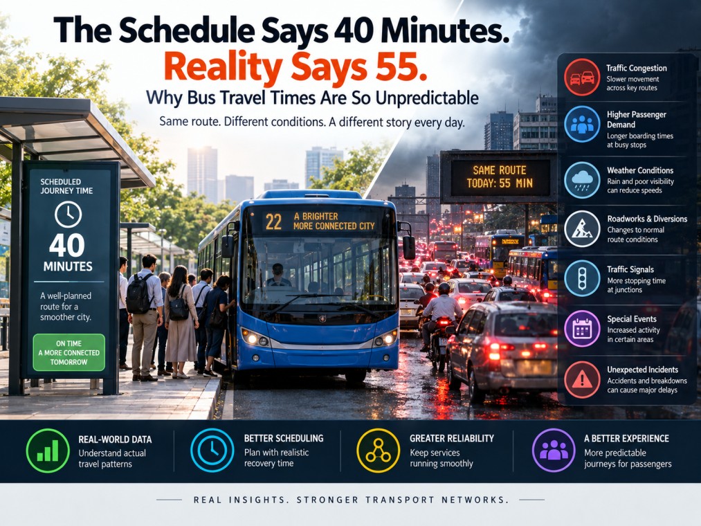
A bus route may be planned to take 40 minutes from one terminal to another. On paper, that sounds straightforward. The timetable is created, vehicles are assigned, drivers are scheduled, and passengers are given expected arrival times.

But once the bus enters the real world, things become less predictable.

The same route might take 38 minutes on one trip, 43 minutes on another, and 55 minutes during the evening peak. Traffic congestion, passenger demand, road conditions, traffic signals, weather, roadworks, and unexpected incidents can all change how long the journey takes.

This raises an important question: if the route remains the same, why does the travel time keep changing?

The answer lies in a fundamental challenge in public transport operations: travel-time variability.

Understanding this phenomenon is essential because a timetable is more than a list of departure and arrival times. It is an operational plan based on assumptions about how vehicles, passengers, and roads will behave throughout the day. When those assumptions do not reflect actual conditions, even a well-designed schedule can become difficult to maintain.

What Is Travel-Time Variability?

Travel-time variability is the difference between the time required to complete the same journey under different conditions.

A bus travelling along the same corridor may encounter completely different circumstances depending on the time of day. Traffic may be light during the middle of the day but extremely heavy during the morning commute. A relatively empty bus may move quickly through its stops, while a crowded vehicle may spend several additional minutes boarding passengers.

For example, a route could have actual journey times of:

• 38 minutes on a quiet trip
• 42 minutes during moderate traffic
• 47 minutes during a busy period
• 55 minutes during severe congestion

The average might provide a useful summary, but it does not tell an operator how predictable the service really is.

This is an important distinction in transit planning. Operators need to understand not only the typical journey duration but also how widely actual travel times vary around that typical value.

Research using Automatic Vehicle Location data from a bus route in Mysore, India, has demonstrated how actual bus travel times can be analysed statistically to understand transit reliability rather than treating journey duration as a fixed figure.

Why the Same Route Takes Different Amounts of Time

Travel time is influenced by a combination of factors rather than a single variable.

Road congestion is one of the most obvious. A bus travelling through a busy commercial corridor may lose several minutes at intersections or in slow-moving traffic.

Passenger activity is another major factor. When many passengers board or alight at the same stop, the vehicle remains stationary for longer. This becomes particularly noticeable at major interchanges, markets, railway stations, schools, and other high-demand locations.

Weather can also affect operations. Heavy rain may reduce road speeds, increase congestion, and make passenger movement around stops slower. Road construction, temporary diversions, accidents, special events, and changes in traffic patterns can introduce further uncertainty.

The route itself also matters. A corridor with many closely spaced stops provides more opportunities for passenger activity to influence the journey.

Research into bus service reliability has identified factors including passenger demand, dwell time, route characteristics, service frequency, and operational irregularity as contributors to variations in bus performance.

The important point is that travel time is not a fixed property of a route. It is the outcome of several changing conditions interacting with one another.

Why Planning Around the Average Can Be Misleading

Suppose historical data shows that a particular route takes an average of 40 minutes.

It may seem logical to create a 40-minute timetable.

However, imagine that the actual journey times vary between 35 and 52 minutes depending on the conditions.

The average may still look acceptable, but a schedule built around 40 minutes will regularly be exposed to delays.

This is why transport planning needs to look beyond averages.

Passengers do not experience an "average journey." They experience a specific trip at a specific time under specific conditions.

For someone travelling to work, arriving in 40 minutes most days but taking 52 minutes on another day can make the service feel unreliable even when the average performance appears reasonable.

This is why reliability and predictability are just as important as speed.

Statistical approaches to public transport reliability increasingly consider the distribution of travel times and the probability of delays rather than relying solely on mean journey duration.

How a Small Delay Can Grow Into an Operational Problem

A few minutes of variation may appear insignificant when looking at a single journey.

In a scheduled operation, however, that difference can have consequences beyond the individual trip.

Imagine a bus leaves the depot five minutes behind schedule. It then loses another three minutes in congestion. At a busy stop, passenger boarding takes four minutes longer than expected.

By the time the bus reaches the end of its route, it is already 12 minutes late.

The next trip was supposed to begin shortly after the vehicle arrived at the terminal. Because the bus is late, some or all of its planned recovery time disappears.

The following journey now begins behind schedule.

If the same conditions continue, the vehicle can carry the delay into subsequent trips.

This is why operators need to consider the entire vehicle duty, rather than looking at each journey as an isolated event.

Passenger Demand Can Change the Journey Itself

One of the most interesting characteristics of bus operations is that passengers can influence the conditions that affect their own journey.

Consider a bus arriving at a busy stop with 40 people waiting.

Boarding takes longer than usual. The bus leaves several minutes later than planned.

The next bus arrives shortly afterwards and finds fewer passengers because many have already boarded the first vehicle.

It spends less time at the stop and may gradually close the gap with the bus ahead.

This interaction between passenger demand, dwell time and vehicle movement can contribute to irregular service patterns and, under certain conditions, bus bunching.

Research into bus reliability has identified passenger demand and dwell time as important factors influencing headway variability and service regularity.

The lesson is important: passenger demand is not just something operators respond to. It can also influence how the service performs.

Why Peak Hours Are Especially Difficult

The difference between a robust schedule and a fragile one often becomes most visible during peak periods.

Morning and evening peaks combine several pressures at once:

• More vehicles on the road
• Higher passenger volumes
• Longer boarding times
• Heavier traffic
• Greater demand at key stops
• More pressure on connecting services

A route that normally takes 40 minutes may require considerably more time during these periods.

If the timetable assumes that the same journey duration applies throughout the day, delays can become a recurring feature rather than an occasional exception.

This does not mean that operators should automatically make every peak-period journey longer. The more useful approach is to understand where and when additional time is actually needed.

Should Operators Simply Add More Time?

At first glance, the solution seems simple: if a journey sometimes takes 55 minutes, schedule it for 55 minutes.

But that creates another problem.

If the bus normally completes the route in 40 minutes, adding 15 minutes to every scheduled trip means that the fleet spends more time completing the same work.

That can reduce vehicle productivity, affect required fleet size and make services slower than necessary during periods when roads are relatively clear.

Operators therefore face a difficult trade-off.

Too little recovery time can reduce reliability. Too much can reduce efficiency.

The objective is not to eliminate every variation. That would be unrealistic.

The objective is to understand the variation well enough to build a timetable that can absorb normal fluctuations without creating unnecessary operating costs.

Where Should Recovery Time Be Added?

Recovery time is the additional flexibility built into an operation to absorb delays before they affect subsequent trips.

However, placing recovery time everywhere is not an efficient solution.

Historical data may show that a particular section of a route consistently experiences congestion between 8 AM and 9 AM. Another part may experience longer boarding times around lunchtime because of high passenger demand.

Instead of treating the entire route as equally unpredictable, planners can identify the sections and time periods where additional flexibility is most valuable.

This creates a more targeted approach to schedule design.

Rather than saying:

"This route needs 10 extra minutes."

the question becomes:

"Where does the variability occur, when does it occur, and how much recovery time is actually needed?"

That is a much more useful way to approach scheduling.

From Assumptions to Actual Data

This is where data-driven planning becomes particularly valuable.

Traditional scheduling can rely heavily on expected journey times and planner experience. Those inputs remain useful, but actual operational data can reveal patterns that are difficult to identify manually.

Historical vehicle-location information can help operators understand how long each section of a route actually takes at different times of day.

Over time, this can reveal:

• Typical travel times
• Peak-period variations
• Locations with recurring delays
• High-dwell-time stops
• Seasonal patterns
• Differences between scheduled and actual performance
• Routes with unusually wide travel-time variation
• Periods where recovery time is regularly consumed

This changes the planning question from "How long should this route take?" to "What range of journey times should we expect under different conditions?"

The second question provides much more useful information for building resilient schedules.

Real-Time Data Adds Another Dimension

Historical information tells operators what usually happens.

Real-time information tells them what is happening right now.

Suppose a route normally takes 42 minutes during the morning peak, but today's traffic conditions indicate that buses are moving considerably slower than usual.

With real-time visibility, an operator can identify the developing issue before it becomes a larger service problem.

Depending on the situation, the response could include adjusting dispatch, reallocating available vehicles, communicating changes to passengers, or making other operational decisions.

The value of real-time information is therefore not simply knowing where a bus is. It is understanding how current conditions differ from the expected operating pattern.

Why This Matters for Indian Cities

Travel-time variability is particularly relevant to Indian urban transport, where buses often operate in complex road environments alongside cars, two-wheelers, auto-rickshaws, commercial vehicles and pedestrians.

Traffic conditions can change quickly, while passenger demand can vary significantly between different parts of the same route.

A timetable that performs well during one period may struggle during another. Special events, school hours, market activity, weather and temporary road restrictions can introduce additional variation.

The Mysore research mentioned earlier provides an example of how actual bus location data from an Indian route can be used to analyse travel-time distributions and transit reliability.

The broader lesson is straightforward: local operating data matters.

A schedule based on assumptions may look efficient.

A schedule based on observed conditions has a better chance of being reliable.

What Operators Should Measure

Understanding variability requires more than checking whether buses are simply "on time."

Operators can examine several dimensions of performance, including:

• Actual travel time by route segment
• Variation by time of day
• Scheduled versus actual arrival times
• Dwell time at individual stops
• Passenger boarding and alighting patterns
• Recovery time available between trips
• Recurring congestion locations
• Trip completion rates
• Headway variation
• Vehicle and driver availability

Taken together, these measures can help identify whether delays are primarily associated with the timetable, traffic conditions, passenger activity, operational constraints, or a combination of factors.

The Goal Is Not Perfect Prediction

No transport operator can predict every traffic incident, passenger surge or road disruption.

Nor should the objective be to create a timetable that assumes everything will happen exactly as expected.

The more practical goal is to understand the range of conditions in which the service operates.

A strong schedule recognises that variation exists. It identifies where that variation is concentrated and provides enough flexibility to handle normal fluctuations without unnecessarily slowing the entire operation.

This is the difference between a timetable that looks efficient on paper and one that is designed for actual operating conditions.

How Technology Can Support Better Scheduling

When route planning, scheduling, fleet information, vehicle locations and operational conditions are viewed together, transport teams can compare planned performance with what is actually happening on the road.

For example, if a particular corridor consistently takes longer than expected during a specific period, the pattern can be identified through historical data rather than being treated as a series of unrelated delays.

The planning process can then become a continuous cycle:

Plan → Operate → Measure → Analyse → Improve

This approach allows schedules to evolve as operating conditions change.

It also helps planners distinguish between an occasional disruption and a recurring structural problem that requires a change to the timetable or operational strategy.

Where RouteSync Fits

This is where connected transport management can support more informed decision-making.

RouteSync, developed by Arena Softwares, brings together capabilities such as route planning, scheduling, fleet management, vehicle monitoring and operational visibility.

The value of connecting these areas is that operators can look beyond individual vehicles and examine how planned schedules compare with actual fleet movement and changing operating conditions.

That can help transport teams identify recurring patterns, respond to developing issues and make better-informed decisions about schedules, resources and service performance.

The Bigger Lesson

A bus timetable is a plan. The road is reality.

Between the two are traffic, passenger demand, weather, road conditions, traffic signals, incidents and countless small variations that change throughout the day.

That is why a route scheduled for 40 minutes can sometimes take 55.

The solution isn't simply to add more time to every journey. It is to understand why travel times vary, where the variation occurs, how frequently it happens, and what effect it has on the wider operation.

With better historical analysis and real-time visibility, operators can build schedules around actual conditions rather than relying entirely on fixed assumptions. They can identify vulnerable sections, place recovery time where it provides the most value, respond to developing problems and improve the reliability of subsequent trips.

Ultimately, reliable public transport is not about making every journey take exactly the same amount of time.

It is about creating a service that is predictable enough for passengers and flexible enough to deal with reality.

Because the best timetable isn't the one that looks perfect on paper. It's the one that continues to work when the city doesn't.